The Line of Best Fit Equation
The line of best fit determined from the least squares method has an equation that tells the story of the relationship between the data points. Line of best fit equations may be determined by computer software models, which include a summary of outputs for analysis, where the coefficients and summary outputs explain the dependence of the variables being tested. The least squares method provides the overall rationale for the placement of the line of best fit among the data points being studied. The “least squares” method is a form of mathematical regression analysis used to determine the line of best fit for a set of data, providing a visual demonstration of the relationship between the data points.
There is a close connection between correlation and the slope of the least square line. It is interesting that the least squares regression line always passes through the point (`x , `y ). The correlation (r) describes the strength of a straight line relationship.
Calculating the Least Squares Regression Line by Hand
The square of the correlation, r2 , is the fraction of the variation in the values of y that is explained by the regression of y on x. Remember, it is a good idea to include r2 as a measure of how successful the regression was in explaining the response when you report a regression line.
Linear regression is basically a mathematical analysis method which considers the relationship between all the data points in a simulation. All these points are based upon two unknown variables; one independent and one dependent. The dependent variable will be plotted on the y-axis and the independent variable will be plotted to the x-axis on the graph of regression analysis. In literal manner, least square method of regression minimizes the sum of squares of errors that could be made based upon the relevant equation.
How do you use least squares method?
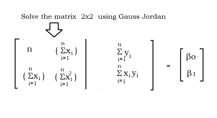
Step 1: Calculate the mean of the x -values and the mean of the y -values. Step 4: Use the slope m and the y -intercept b to form the equation of the line. Example: Use the least square method to determine the equation of line of best fit for the data.
It is used in regression analysis, often in nonlinear regression modeling in which a curve is fit into a set of data. The term “least squares” is used because it is the smallest sum of squares of errors, which is also called the “variance”. When calculating least squares regressions by hand, the first step is to find the means of the dependent and independent variables.
How do you calculate least squares regression?
The least squares method is a statistical procedure to find the best fit for a set of data points by minimizing the sum of the offsets or residuals of points from the plotted curve. Least squares regression is used to predict the behavior of dependent variables.
Regression Basics for Business Analysis
Each point of data represents the relationship between a known independent variable and an unknown dependent variable. Least squares regression analysis or linear regression method is deemed to be the most accurate and reliable method to divide the company’s mixed cost into its fixed and variable cost components. This is because this method takes into account all the data points plotted on a graph at all activity levels which theoretically draws a best fit line of regression. However, if the errors are not normally distributed, a central limit theorem often nonetheless implies that the parameter estimates will be approximately normally distributed so long as the sample is reasonably large. For this reason, given the important property that the error mean is independent of the independent variables, the distribution of the error term is not an important issue in regression analysis.
- Linear regression is basically a mathematical analysis method which considers the relationship between all the data points in a simulation.
For example, suppose there is a correlation between deaths by drowning and the volume of ice cream sales at a particular beach. Yet, both the number of people going swimming and the volume of ice cream sales increase as the weather gets hotter, and presumably the number of deaths by drowning is correlated with the number of people going swimming. It is possible that an increase in swimmers causes both the other variables to increase. In 1810, after reading Gauss’s work, Laplace, after proving the central limit theorem, used it to give a large sample justification for the method of least squares and the normal distribution. We should distinguish between “linear least squares” and “linear regression”, as the adjective “linear” in the two are referring to different things.
This approach does commonly violate the implicit assumption that the distribution of errors is normal, but often still gives acceptable results using normal equations, a pseudoinverse, etc. Depending on the type of fit and initial parameters chosen, the nonlinear fit may have good or poor convergence properties. If uncertainties (in the most general case, error ellipses) are given for the points, points can be weighted differently in order to give the high-quality points more weight. The linear least squares fitting technique is the simplest and most commonly applied form of linear regression and provides a solution to the problem of finding the best fitting straight line through a set of points. For this reason, standard forms for exponential, logarithmic, and powerlaws are often explicitly computed.
This method of regression analysis begins with a set of data points to be plotted on an x- and y-axis graph. An analyst using the least squares method will generate a line of best fit that explains the potential relationship between independent and dependent variables. “Best” means that the least squares estimators of the parameters have minimum variance. The assumption of equal variance is valid when the errors all belong to the same distribution. In regression analysis, dependent variables are illustrated on the vertical y-axis, while independent variables are illustrated on the horizontal x-axis.
These designations will form the equation for the line of best fit, which is determined from the least squares method. For nonlinear least squares fitting to a number of unknown parameters, linear least squares fitting may be applied iteratively to a linearized form of the function until convergence is achieved. However, it is often also possible to linearize a nonlinear function at the outset and still use linear methods for determining fit parameters without resorting to iterative procedures.
The formulas for linear least squares fitting were independently derived by Gauss and Legendre. The researcher specifies an empirical model in regression analysis. A very common model is the straight line model, which is used to test if there is a linear relationship between independent and dependent variables. The variables are said to be correlated if a linear relationship exists.
If the probability distribution of the parameters is known or an asymptotic approximation is made, confidence limits can be found. Similarly, statistical tests on the residuals can be conducted if the probability distribution of the residuals is known or assumed. We can derive the probability distribution of any linear combination of the dependent variables if the probability distribution of experimental errors is known or assumed. Inferring is easy when assuming that the errors follow a normal distribution, consequently implying that the parameter estimates and residuals will also be normally distributed conditional on the values of the independent variables.
Specifically, it is not typically important whether the error term follows a normal distribution. Here a model is fitted to provide a prediction rule for application in a similar situation to which the data used for fitting apply. Here the dependent variables corresponding to such future application would be subject to the same types of observation error as those in the data used for fitting.
The former refers to a fit that is linear in the parameters, and the latter refers to fitting to a model that is a linear function of the independent variable(s). Linear regression assumes a linear relationship between the independent and dependent variable.
In standard regression analysis that leads to fitting by least squares there is an implicit assumption that errors in the independent variable are zero or strictly controlled so as to be negligible. Regression is one of the most common statistical settings and least squares is the most common method for fitting a regression line to data.
What Is the Least Squares Method?
It is therefore logically consistent to use the least-squares prediction rule for such data. The least squares approach limits the distance between a function and the data points that the function explains.