The easiest way to apply Accounting is to use the Number Format menu on the ribbon. When you apply the Currency format to a number, the currency symbol appears right next to the first digit in the cell. You can specify the number of decimal places that you want to use, whether you want to use a thousands separator, and how you want to display negative numbers. In the Format Cells dialog box, in the Category list, click Currency or Accounting.
Like the Currency format, the Accounting format is used for monetary values. But, this format aligns the currency symbols and decimal points of numbers in a column. In addition, the Accounting format displays zeros as dashes and negative numbers in parentheses. Like the Currency format, you can specify how many decimal places you want and whether to use a thousands separator. You can’t change the default display of negative numbers unless you create a custom number format.
How to Apply Accounting Number Format in Excel
You also will need to select a different number format for the date column and other columns that do not require accounting formatting for cells. Excel uses the “General” number format as the default number format for spreadsheet cells. Data typed into the default formatted cell are usually left as entered with no added formatting.
Create a workbook template with specific currency formatting settings
1) In order to apply Accounting format, select the range and right-click and choose Format Cells. When it comes to setting the currency symbol for the Accounting format, we have some new options. There are shortcuts on the ribbon for several common currency symbols, and we can use these shortcuts to for the British Pound and Euro. In this lesson we’ll take a look at the Accounting format. Like the Currency format, the Accounting number format is designed for numbers with currency symbols.
Format numbers as currency
Notice that the currency symbols are not right next to the numbers. To change some of the currency numbers to another type of currency, such as Euros, select the cells you want to change.
The difference between the Accounting format and the Currency format is that the Accounting format puts the dollar sign for example, at the far left end of the cell, and displays zero as a dash. So, let’s look at a simple example in order to see how to apply Accounting number format in Excel. If you want to display numbers as monetary values, you must format those numbers as currency. To do this, you apply either the Currency or Accounting number format to the cells that you want to format. The number formatting options are available on the Home tab, in the Number group.
What is accounting format?
Accounting. Like the Currency format, the Accounting format is used for monetary values. But, this format aligns the currency symbols and decimal points of numbers in a column. In addition, the Accounting format displays zeros as dashes and negative numbers in parentheses.
If Excel displays ##### in a cell after you apply currency formatting to your data, the cell probably isn’t wide enough to display the data. To expand the column width, double-click the right boundary of the column that contains the cells with the ##### error. You can also drag the right boundary until the columns are the size that you want. After you create a table, Microsoft Office Word 2007 offers you many ways to format that table. It includes Classic Menu for Word, Excel, PowerPoint, OneNote, Outlook, Publisher, Access, InfoPath, Visio and Project 2010, 2013, 2016, 2019 and 365.
Are you looking for a way to shorten the time you spend on your spreadsheets? Instead of entering all your data manually, you can use the AutoFill feature to fill cells with data that follows a pattern or that is based on data in other cells.
Exceljet
However, this is the “Accounting Number Format”, not the standard currency format. Excel has several built-in formulas for financial calculations, such as asset depreciation and cash flow. Excel users create formulas to accomplish the necessary calculations.
Unfortunately, Word does not allow you to do this type of formatting directly. Change the number format in an existing spreadsheet by changing the format in cell 1A and using the format painter to change the format in a range of cells.
Before you do anything else, make sure the numbers in question are formatted as currency. The Currency format and the Accounting format in Excel are very similar to each other. Applying the Accounting format is simple and straightforward in Excel.
- You may have noticed a drop-down list in the “Number” section of the “Home” tab that has a currency symbol on it.
- However, this is the “Accounting Number Format”, not the standard currency format.
This allows users to read and spell the numbers incorrect form. To enable the comma in any cell select Format Cells from the right-click menu and from Number section check the box of Use 1000 separator . We can also use the Home menu ribbons’ Commas Style under the number section. We can also even use short cut keys by pressing ALT + H + K simultaneously to apply comma style.
The accounting format in Microsoft Excel 2010 is very similar to the currency format—both display the currency symbol next to every number. 2) In the Format Cells Dialog box, with the Number Tab selected, choose Accounting and accept the options shown below and click Ok.

The numbers in the selected cells are all formatted as currency with Windows’ default currency symbol applied. Those who are familiar with the rich formatting features of Excel may long for a way to format numbers in a Word table just as easily. For instance, you may have a column of numbers that you want to format as currency, complete with the dollar sign.
Brings the familiar classic menus and toolbars back to Microsoft Office 2007, 2010, 2013, 2016, 2019 and 365. You can use Office 2007/2010/2013/2016 immediately without any training. Supports all languages, and all new commands of 2007, 2010, 2013, 2016, 2019 and 365 have been added into the classic interface. Then, select “Currency” from the “Number Format” drop-down list in the “Number” section of the “Home” tab. Excel attempts to guess which cells you want to include in the function by looking for ranges that are adjacent to the selected cell and that contain numeric data.
You may have noticed a drop-down list in the “Number” section of the “Home” tab that has a currency symbol on it. This may seem like an easier way to change the currency symbol for the selected cells.
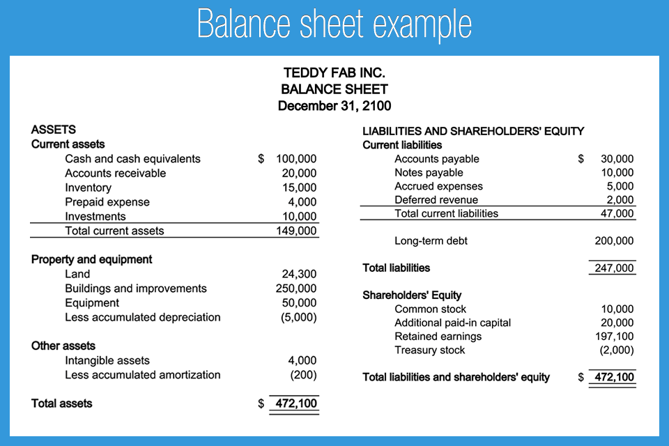
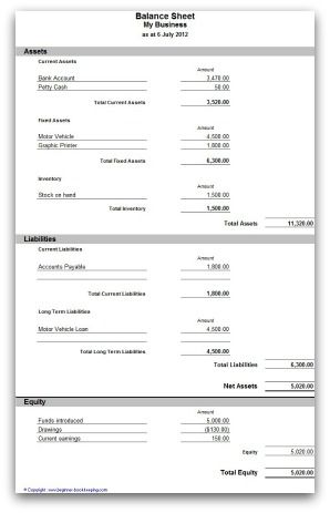
One can use the Accounting format when compiling financial statements, balance sheets and for other Accountancy related purposes. To set a currency symbol of None, or to set other currencies, visit the Format Cells dialog box. Then let’s apply the Accounting format to the columns C through H.
Instead of using the default number format, you can select the accounting number format for your spreadsheet. Now let’s select cells in column D check the options available for Accounting in the Format Cells dialog box. Like the Currency format, the Accounting format provides options for decimal places and a currency symbol, and it automatically uses a comma to separate thousands. Unlike Currency, there are no options for negative numbers. The Accounting format places parentheses around all negative numbers by default.
You can also change the number of decimal places and the format of negative numbers on the “Number” tab on the “Format Cells” dialog box. …you’ll get Euro symbols on your numbers, but they will display in the accounting format, which aligns the decimal points in a column.
If you’re working with different currencies in one Excel spreadsheet, you’ll need to change the currency symbol on certain cells, without affecting other cells. When you format your numbers as “Currency”, you can easily use multiple currency symbols in the same Excel spreadsheet. The accounting format lines up the left-aligned currency symbols and the decimal points, no matter the number of decimal places, throughout a column, and places parenthesis around negative numbers. Comma style is Excel mainly used for numbers to distinguish the different lengths like hundreds, thousands, millions, etc.
Select the top-left cell in the range of cells that you want to change to the accounting format. Scroll the spreadsheet, using the scroll bars on the right and bottom edges of the spreadsheet, so that you can see the bottom-right cell of your desired range. Hold “Shift” and click this cell to select the entire range. The Accounting Format is similar to the Currency format and can be applied to numbers where needed.
The main difference between Currency and Accounting formats is that Accounting aligns currency symbols to the left in each cell, and displays zero values with a hypen. Select the specific cells or columns you want to format, and then apply currency formatting to them.
After applying the accounting format to spreadsheet cells, you will need to continue formatting your spreadsheet for use as an accounting ledger. Include column headings– such as date, amount and balance–and enter formulas in the cells that will perform calculations.
